Tuesday, June 25, 2013
Chord-changer Javascript
I have written a Javascript program to transpose the guitar chords for a song into a different key. In the lyrics of the song, the guitar chords are supposed to be between <sup> and </sup>. You can try it at Myanmar Lyrics by clicking the Key Up and Key Down buttons. The codes are shown below.


Saturday, June 15, 2013
Algorithm, Program and Calculation of Myanmar Calendar
မြန်မာဘာသာ ဖြင့်ဖတ်ရန်
An easier and faster modern method to calculate a past, present or future date in the Myanmar calendar (the Burmese calendar) is presented. The constants, formulas and steps are clearly defined to derive all the essential elements of the Myanmar calendar such as Myanmar year, Myanmar month, waxing or waning moon and day. Unlike the existing methods, this method is easy even for a person who is not familiar with the Myanmar calendar and its terms.
An easier and faster modern method to calculate a past, present or future date in the Myanmar calendar (the Burmese calendar) is presented. The constants, formulas and steps are clearly defined to derive all the essential elements of the Myanmar calendar such as Myanmar year, Myanmar month, waxing or waning moon and day. Unlike the existing methods, this method is easy even for a person who is not familiar with the Myanmar calendar and its terms.
Thursday, February 28, 2013
Non-inverting Amplifier Using op-amp
When PiezoDrive PDX 150 amplifier that I used to drive a piezoelectric actuator was damaged, I need to find a way to use an existing spare amplifier. The spare amplifier shown in the following figure has input voltage -2 V to 12 V and output voltage -20 V to 120 V. Its gain is only 10 while the damaged one is 20. Therefore, I decided to design and use an additional preamplifier with gain 2.

The input to that amplifier is -1 V to 6 V and its output shold be -2 V to 12 V. Since I need non-inverted output, I have used an op-amp with non-inverting configuration. I have also used a trimmer so that it is possible to fine tune the gain. Readily available LM358N op-amp IC is arbitrarily picked up. The schematic circuit diagram and resulting amplifier using available components in our lab is shown below. Since the non-inverting amplifier has very high input impedance, I have used additional 56k resister to prevent it from floating.


When tuning the amplifier to get exact gain of 2, it looked unreliable to use peak to peak readings from oscilloscope. That was why, I had to think of an alternative way to achieve it. I set channel 1 which was connected to output of the amplifier to 10 V per division and I set channel 2 which was connected to input of the implifier to 5 V per division. After that, I calibrated the trimmer to get identical waves at the screen :P


The input to that amplifier is -1 V to 6 V and its output shold be -2 V to 12 V. Since I need non-inverted output, I have used an op-amp with non-inverting configuration. I have also used a trimmer so that it is possible to fine tune the gain. Readily available LM358N op-amp IC is arbitrarily picked up. The schematic circuit diagram and resulting amplifier using available components in our lab is shown below. Since the non-inverting amplifier has very high input impedance, I have used additional 56k resister to prevent it from floating.


When tuning the amplifier to get exact gain of 2, it looked unreliable to use peak to peak readings from oscilloscope. That was why, I had to think of an alternative way to achieve it. I set channel 1 which was connected to output of the amplifier to 10 V per division and I set channel 2 which was connected to input of the implifier to 5 V per division. After that, I calibrated the trimmer to get identical waves at the screen :P

Wednesday, February 6, 2013
TRIAC Power Control Circuit
My vacuum cleaner was faulty. I thought the reason might be blown fuse and I tried to fix it. Unfortunately, I could not find any fuse either in machine or connector. I then thought that the reason might be the faulty power control circuit. Therefore, I tried to bypass the control circuit by directly connecting power and motor. But it did not work. Finally, I successfully solved the problem by throwing the old one and buying a new vacuum cleaner :P I kept the power control circuit and tried to trace it when I was free. It uses a simple RC circuit and a DIAC to make a phase lag in firing the TRIAC. The circuit is quite simple and it is shown below.


Monday, January 21, 2013
k-means clustering using custom distance measuring method
I have developed a MATLAB function to perform k-means clustering which enables custom distance measuring method. For example, to sort out histograms, chi-square distance may be more suitable. The following example function uses chi-square distance and you can replace it with any distance measurement method.


%k-means test program
X = [randn(100,2)+ones(100,2);...
     randn(100,2)-ones(100,2)];

[idx,ctrs] = KMeansCustom(X,2);
%[idx,ctrs] = kmeans(X,2);

plot(X(idx==1,1),X(idx==1,2),'r.','MarkerSize',12)
hold on
plot(X(idx==2,1),X(idx==2,2),'b.','MarkerSize',12)
plot(ctrs(:,1),ctrs(:,2),'kx',...
     'MarkerSize',12,'LineWidth',2)
legend('Cluster 1','Cluster 2','Centroids',...
       'Location','NW')
function [Idx,C]=KMeansCustom(X,k)
%KMeansCustom partitions the points in the n-by-d data matrix X into k clusters.
%[Idx,C]= KMeansCustom(X,k) returns
%n-by-1 vector IDX containing the cluster indices of each point and
%k-by-d matrix C containing the k cluster centroid locations.
%For n sample points with d dimensions in each point, X has n rows and d columns.
%File name: KMeanCustom.m
%Author: Yan Naing Aye
%Website: http://cool-emerald.blogspot.sg/


%%%%%%%%%%%%%%%%%%%%%%%%%%%%%%%%%%%%%%%%%%%%%%%%%%%%%%%%%%%
%Define maximum number of iterations
MaxIter=500;
%%%%%%%%%%%%%%%%%%%%%%%%%%%%%%%%%%%%%%%%%%%%%%%%%%%%%%%%%%%
[n,d]=size(X);
k=round(k);
%%%%%%%%%%%%%%%%%%%%%%%%%%%%%%%%%%%%%%%%%%%%%%%%%%%%%%%%%%%
%step1 :arbitrarily choose k samples as the initial cluster centers
p=randperm(n);
Mu=X(p(1:k),:);
D=zeros(k,d);
for t=1:MaxIter
 %step2:distribute the samples X  to the clusters
 for j=1:k
        for i=1:n
            D(j,i)=ChiDist(X(i,:),Mu(j,:));%Use custom distance
        end
 end
 [ValMin,IndexMin]=min(D);
 %%%%%%%%%%%%%%%%%%%%%%%%%%%%%%%%%%%%%%%%%%%%%%%%%%%%%%%%%%%
 %step 3: update the cluster centers
    OldMu=Mu;
 for i=1:k
        Mu(i,:)=mean(X(IndexMin==i,:));
 end
 %%%%%%%%%%%%%%%%%%%%%%%%%%%%%%%%%%%%%%%%%%%%%%%%%%%%%%%%%%%%%
 %step4 :check convergence
 if sum(sum(abs(OldMu-Mu))) == 0 %< 1e-9
        break
 end
end
Idx=IndexMin';
C=Mu;
function d=ChiDist(v1,v2)
    dv=(v1-v2).^2;
    sv=abs(v1)+abs(v2);
    %------------------------------------------------------
    %eliminate zero denominator
    sv(sv==0)=1e-9;
    %------------------------------------------------------
    d=sum(dv./sv)./2;
end
Amplitude spectrum of a signal using Fourier transform
I have developed a MATLAB function to calculate amplitude spectrum of a signal using Fourier transform. Example usage of the function and implementation is shown below. Another example MATLAB program using built in function fft is also demonstrated. I hope they will be helpful for those who want to find amplitude spectrum or power spectrum of a signal.
%Example MATLAB code to test function FX
Fs=100;
t=(0:1/Fs:1-1/Fs)';
x=2*cos(2*pi*5*t)+sin(2*pi*10*t);
[f a]=FX(x,Fs);
plot(f,a);
function [f a]=FX(x,fs)
%Calculates amplitude spectrum of a signal x using Fourier transform
%[f a]=FX(x,fs)
%Input: x=signal, fs = sampling rate
%Output: f = frequency axis, a = amplitude spectrum
%File name: FX.m
%Author: Yan Naing Aye
%Website: http://cool-emerald.blogspot.sg/

dT = 1/fs;
N=length(x);
dF=1/(N*dT);
NF=fs/2;%Nyquist Freq
%You can always limit freq range for faster performance
%NF=20;
t=(0:dT:(N-1)*dT)';
f=(0:dF:NF)';
a=f;%initialize a
a(1)=mean(x);
for i=2 : length(a)
    b=(2*mean(x.*cos(2*pi*dF*(i-1)*t)));
    c=(2*mean(x.*sin(2*pi*dF*(i-1)*t)));
    a(i)=sqrt(b^2+c^2);
end
%MATLAB program to calculates amplitude spectrum of a signal x using fft
%Author: Yan Naing Aye
%Website: http://cool-emerald.blogspot.sg/

Fs=100;
t=(0:1/Fs:1-1/Fs)';
x=2*cos(2*pi*5*t)+sin(2*pi*10*t);
L=length(x);

A=2*abs(fft(x)/L);
A=A(1:Fs/2+1);
f = Fs/2*linspace(0,1,Fs/2+1);
plot(f,A);
Sunday, January 13, 2013
Changing sampling rate using quadratic regression
I want to change sampling rate of a signal from 333Hz to 5000Hz. To get a smoother result, I have implemented second order hold system instead of popular zero order hold (ZOH) system. This approach can also be used for down sampling. Another possible application is to filter out noise without introducing phase delay. And it can be useful for real-time application.
Approach 1: Quadratic regression
Quadratic function is defined as
$$f=w_0+w_1 x + w_2 x^2$$
Then, cost function to be minimized is defined as
$$J(w)=\frac{1}{2}\sum_{i=1}^{n}(y_i-f_i)^2$$
$$J(w)=\frac{1}{2}\sum_{i=1}^{n}(y_i-w_0+w_1 x_i + w_2 x_i^2)^2$$
Optimal weights can be found by differentiating the cost function and setting them to zero.
$$\frac{\partial J(w)}{\partial w_0}=0$$
$$-\sum_{i=1}^{n}(y_i-w_0+w_1 x_i + w_2 x_i^2)=0$$
$$w_0\sum_{i=1}^{n}1+w_1\sum_{i=1}^{n}x_i+w_2\sum_{i=1}^{n}x_i^2=\sum_{i=1}^{n}y_i$$
Similarly, differentiating with w1 and w2 gives,
$$w_0\sum_{i=1}^{n}x_i+w_1\sum_{i=1}^{n}x_i^2+w_2\sum_{i=1}^{n}x_i^3=\sum_{i=1}^{n}y_i x_i$$
$$w_0\sum_{i=1}^{n}x_i^2+w_1\sum_{i=1}^{n}x_i^3+w_2\sum_{i=1}^{n}x_i^4=\sum_{i=1}^{n}y_i x_i^2$$
When these three equations are written in matrix form.
$$ \begin{bmatrix} \sum_{i=1}^{n}1 & \sum_{i=1}^{n}x_i & \sum_{i=1}^{n}x_i^2 \\ \sum_{i=1}^{n}x_i & \sum_{i=1}^{n}x_i^2 & \sum_{i=1}^{n}x_i^3 \\ \sum_{i=1}^{n}x_i^2 & \sum_{i=1}^{n}x_i^3 & \sum_{i=1}^{n}x_i^4 \end{bmatrix} \begin{bmatrix} w_0 \\ w_1 \\ w_2 \end{bmatrix} = \begin{bmatrix} \sum_{i=1}^{n}y_i \\ \sum_{i=1}^{n}y_i x_i \\ \sum_{i=1}^{n}y_i x_i^2 \end{bmatrix} $$
$$\mathbf{A}\mathbf{W}=\mathbf{B}$$
$$\mathbf{W}=\mathbf{A}^{-1}\mathbf{B}$$
Approach 2: Three equations
In our case, we can use only the last three points and we can get three equations from these three points.

$$y_1=w_0+w_1 x_1 + w_2 x_1^2$$
$$y_2=w_0+w_1 x_2 + w_2 x_2^2$$
$$y_3=w_0+w_1 x_3 + w_2 x_3^2$$
$$ \begin{bmatrix} 1 & x_1 & x_1^2 \\ 1 & x_2 & x_2^2 \\ 1 & x_3 & x_3^2 \end{bmatrix} \begin{bmatrix} w_0 \\ w_1 \\ w_2 \end{bmatrix} = \begin{bmatrix} y_1 \\ y_2 \\ y_3 \end{bmatrix} $$
$$\mathbf{A}\mathbf{W}=\mathbf{B}$$
$$\mathbf{W}=\mathbf{A}^{-1}\mathbf{B}$$
Approach 3: Two equations
If we define x1=-1, x2=0, and x3=1, y2 is equal to w0. And,
$$y_1=y_2-w_1+ w_2$$
$$y_3=y_2+w_1+ w_2$$
$$ \begin{bmatrix} -1 & 1 \\ 1 & 1 \end{bmatrix} \begin{bmatrix} w_1 \\ w_2 \end{bmatrix} = \begin{bmatrix} y_1-y_2 \\ y_3-y2 \end{bmatrix} $$
$$ \begin{bmatrix} w_1 \\ w_2 \end{bmatrix} = \begin{bmatrix} -0.5 & 0.5 \\ 0.5 & 0.5 \end{bmatrix} \begin{bmatrix} y_1-y_2 \\ y_3-y2 \end{bmatrix} $$
Then, we have
$$w_0=y_2$$
$$w_1=-0.5(y_1-y_2)+0.5(y_3-y2)$$
$$w_2=0.5(y_1-y_2)+0.5(y_3-y2)$$
I have tested the above three approaches using MatLab and it is shown below.
 The implementation of this method in LabVIEW using C code is shown in the following figure.
 The first two approaches involve finding inverse of a 3x3 matrix and I have developed a C program as shown below.
Approach 1: Quadratic regression
Quadratic function is defined as
$$f=w_0+w_1 x + w_2 x^2$$
Then, cost function to be minimized is defined as
$$J(w)=\frac{1}{2}\sum_{i=1}^{n}(y_i-f_i)^2$$
$$J(w)=\frac{1}{2}\sum_{i=1}^{n}(y_i-w_0+w_1 x_i + w_2 x_i^2)^2$$
Optimal weights can be found by differentiating the cost function and setting them to zero.
$$\frac{\partial J(w)}{\partial w_0}=0$$
$$-\sum_{i=1}^{n}(y_i-w_0+w_1 x_i + w_2 x_i^2)=0$$
$$w_0\sum_{i=1}^{n}1+w_1\sum_{i=1}^{n}x_i+w_2\sum_{i=1}^{n}x_i^2=\sum_{i=1}^{n}y_i$$
Similarly, differentiating with w1 and w2 gives,
$$w_0\sum_{i=1}^{n}x_i+w_1\sum_{i=1}^{n}x_i^2+w_2\sum_{i=1}^{n}x_i^3=\sum_{i=1}^{n}y_i x_i$$
$$w_0\sum_{i=1}^{n}x_i^2+w_1\sum_{i=1}^{n}x_i^3+w_2\sum_{i=1}^{n}x_i^4=\sum_{i=1}^{n}y_i x_i^2$$
When these three equations are written in matrix form.
$$ \begin{bmatrix} \sum_{i=1}^{n}1 & \sum_{i=1}^{n}x_i & \sum_{i=1}^{n}x_i^2 \\ \sum_{i=1}^{n}x_i & \sum_{i=1}^{n}x_i^2 & \sum_{i=1}^{n}x_i^3 \\ \sum_{i=1}^{n}x_i^2 & \sum_{i=1}^{n}x_i^3 & \sum_{i=1}^{n}x_i^4 \end{bmatrix} \begin{bmatrix} w_0 \\ w_1 \\ w_2 \end{bmatrix} = \begin{bmatrix} \sum_{i=1}^{n}y_i \\ \sum_{i=1}^{n}y_i x_i \\ \sum_{i=1}^{n}y_i x_i^2 \end{bmatrix} $$
$$\mathbf{A}\mathbf{W}=\mathbf{B}$$
$$\mathbf{W}=\mathbf{A}^{-1}\mathbf{B}$$
Approach 2: Three equations
In our case, we can use only the last three points and we can get three equations from these three points.

$$y_1=w_0+w_1 x_1 + w_2 x_1^2$$
$$y_2=w_0+w_1 x_2 + w_2 x_2^2$$
$$y_3=w_0+w_1 x_3 + w_2 x_3^2$$
$$ \begin{bmatrix} 1 & x_1 & x_1^2 \\ 1 & x_2 & x_2^2 \\ 1 & x_3 & x_3^2 \end{bmatrix} \begin{bmatrix} w_0 \\ w_1 \\ w_2 \end{bmatrix} = \begin{bmatrix} y_1 \\ y_2 \\ y_3 \end{bmatrix} $$
$$\mathbf{A}\mathbf{W}=\mathbf{B}$$
$$\mathbf{W}=\mathbf{A}^{-1}\mathbf{B}$$
Approach 3: Two equations
If we define x1=-1, x2=0, and x3=1, y2 is equal to w0. And,
$$y_1=y_2-w_1+ w_2$$
$$y_3=y_2+w_1+ w_2$$
$$ \begin{bmatrix} -1 & 1 \\ 1 & 1 \end{bmatrix} \begin{bmatrix} w_1 \\ w_2 \end{bmatrix} = \begin{bmatrix} y_1-y_2 \\ y_3-y2 \end{bmatrix} $$
$$ \begin{bmatrix} w_1 \\ w_2 \end{bmatrix} = \begin{bmatrix} -0.5 & 0.5 \\ 0.5 & 0.5 \end{bmatrix} \begin{bmatrix} y_1-y_2 \\ y_3-y2 \end{bmatrix} $$
Then, we have
$$w_0=y_2$$
$$w_1=-0.5(y_1-y_2)+0.5(y_3-y2)$$
$$w_2=0.5(y_1-y_2)+0.5(y_3-y2)$$
I have tested the above three approaches using MatLab and it is shown below.
%-------------------------------------------------------------------------
clc;
close all;
clear all;
%-------------------------------------------------------------------------
% y= w0 + w1*x + w2* x^2;
%-------------------------------------------------------------------------
%Got x and y
x=[-1 0 1]';
Wo=[4 3 2]';
y=Wo(1)+Wo(2)*x+Wo(3).*x.*x;

%-------------------------------------------------------------------------
%Approach 1
%Polynomial regression of order 2
%For n=3
S1=3;
Sx=sum(x);
Sx2=sum(x.*x);
Sx3=sum(x.*x.*x);
Sx4=sum(x.*x.*x.*x);
Sy=sum(y);
Syx=sum(y.*x);
Syx2=sum(y.*x.*x);

P=[S1 Sx Sx2; Sx Sx2 Sx3; Sx2 Sx3 Sx4];
B=[Sy Syx Syx2]';
%P1=P^(-1);
W1=P\B

%-------------------------------------------------------------------------
%Approach 2
%Linear equations
A=[1 x(1) x(1)*x(1);1 x(2) x(2)*x(2); 1 x(3) x(3)*x(3)];
W2=A\y
%-------------------------------------------------------------------------
%Approach 3
%Only 2 linear equations
w0=y(2);
w1=-0.5*( y(1)- y(2))+0.5*( y(3)- y(2));
w2=0.5*( y(1)- y(2))+0.5*(y(3)- y(2));
W3=[w0 w1 w2]'
%-------------------------------------------------------------------------
The following figure shows the result of using this method (blue color plot) compare to ordinary zero order hold (black color plot). This method gives much more smoother result but it should be noted that it introduces one sample delay.


#include#include main() { float M[3][3]={{3,0,2},{0,2,0},{2,0,2}}; //initialize a 3x3 matrix float N[3][3]={{0,0,0},{0,0,0},{0,0,0}}; //allocate for inverse int i,j; float d; //------------------------------------------------------------------------- N[0][0]=(M[1][1]*M[2][2]-M[2][1]*M[1][2]); N[1][0]=-(M[1][0]*M[2][2]-M[2][0]*M[1][2]); N[2][0]=(M[1][0]*M[2][1]-M[1][1]*M[2][0]); d=M[0][0]*N[0][0]+M[0][1]*N[1][0]+M[0][2]*N[2][0]; N[0][0]/=d; N[1][0]/=d; N[2][0]/=d; N[0][1]=-(M[0][1]*M[2][2]-M[0][2]*M[2][1])/d; N[1][1]=(M[0][0]*M[2][2]-M[0][2]*M[2][0])/d; N[2][1]=-(M[0][0]*M[2][1]-M[0][1]*M[2][0])/d; N[0][2]=(M[0][1]*M[1][2]-M[0][2]*M[1][1])/d; N[1][2]=-(M[0][0]*M[1][2]-M[0][2]*M[1][0])/d; N[2][2]=(M[0][0]*M[1][1]-M[0][1]*M[1][0])/d; //------------------------------------------------------------------------- //print 3x3 matrix for(i=0;i<3;i++) { for(j=0;j<3;j++) printf("%3.4f ",N[i][j]); printf("\n"); } getch(); return 0; }
Wednesday, January 9, 2013
Rotations in 3D space using Euler angles
Rotations in 3D space to relate body reference frame of a device to world reference frame using an Euler angle sequence are discussed.
Euler stated that
Any two independent orthonormal coordinate frames can be related by a sequence of rotations (not more than three) about coordinate axes, where no two successive rotations may be about the same axis.
The illustration of the world reference frame, {M}, and the body reference frame, {B}, is shown in the following figure.

Pan angle rotation, α, is acquired using computer vision. And, tilt angle rotation, β, and roll angle rotation, γ, are acquired by sensing the gravity, g, using onboard accelerometers. Let us consider the roll angle first, assuming there are no pan and tilt angles. When the roll angle, γ, is zero Y-axis is upward vertical and X-axis is horizontal pointing according to right handed rule. The gravity sensed by X-axis accelerometer and Y-axis accelerometer are denoted by gx and gy respectively. The definition of the roll angle is illustrated in the following figure.
 The roll angle, γ, is calculated as
$$ \gamma = \tan^{-1}\frac{gx}{gy} $$.
Then, it is checked for second and third quadrants as
$$ \mathbf{R}_{\gamma}= \begin{bmatrix} \cos(\gamma) & -\sin(\gamma) & 0 \\ \sin(\gamma) & \cos(\gamma) & 0 \\ 0 & 0 & 1 \end{bmatrix}$$
After the roll angle is corrected, let us consider for tilt angle. The definition of the tilt angle is illustrated in the following figure.
 The tilt angle, β, can be calculated from Y and Z components of the gravity. It is important to note that these gravity component values should be in the roll angle rotated frame.
The new values for the gravity components are obtained as
The tilt angle, β, can be calculated from Y and Z components of the gravity. It is important to note that these gravity component values should be in the roll angle rotated frame.
The new values for the gravity components are obtained as
$$ \begin{bmatrix} gx2 \\ gy2 \\ gz2 \end{bmatrix} = \mathbf{R}_{\gamma} \begin{bmatrix} gx \\ gy \\ gz \end{bmatrix} $$
The tilt angle, β, is calculated as
$$\beta = \tan^{-1}\frac{gy2}{gz2} $$.
Then, it is checked for second and third quadrants as
$$ \mathbf{R}_{\beta}= \begin{bmatrix} 1 & 0 & 0\\ 0 & \cos(\gamma) & -\sin(\gamma) \\ 0 & \sin(\gamma) & \cos(\gamma) \end{bmatrix}$$
Similarly, calculation of the pan angle rotation matrix, Rα, and description of pan angle definition are as follows.
$$ \mathbf{R}_{\alpha}= \begin{bmatrix} \cos(\alpha) & -\sin(\alpha) & 0 \\ \sin(\alpha) & \cos(\alpha) & 0 \\ 0 & 0 & 1 \end{bmatrix}$$
 The product of rotation matrices is itself a rotation matrix.
$$ \mathbf{R}=\mathbf{R}_{\alpha} \mathbf{R}_{\beta} \mathbf{R}_{\gamma}$$
The product of rotation matrices is itself a rotation matrix.
$$ \mathbf{R}=\mathbf{R}_{\alpha} \mathbf{R}_{\beta} \mathbf{R}_{\gamma}$$
And, M=RB
Since R is a rotation matrix, inverse of R is obtained by transposing R. The implementation of this 3D rotation in LabVIEW using MabLab code is shown in the following figure.

Quaternion algebra is also easy and popular approach for such 3D transformation.
Reference:
Kuipers, Jack B., Quaternions and rotation sequences : a primer with applications to orbits, aerospace, and virtual reality, Princeton University Press, 1999, ISBN: 0691058725.
Any two independent orthonormal coordinate frames can be related by a sequence of rotations (not more than three) about coordinate axes, where no two successive rotations may be about the same axis.
The illustration of the world reference frame, {M}, and the body reference frame, {B}, is shown in the following figure.

Pan angle rotation, α, is acquired using computer vision. And, tilt angle rotation, β, and roll angle rotation, γ, are acquired by sensing the gravity, g, using onboard accelerometers. Let us consider the roll angle first, assuming there are no pan and tilt angles. When the roll angle, γ, is zero Y-axis is upward vertical and X-axis is horizontal pointing according to right handed rule. The gravity sensed by X-axis accelerometer and Y-axis accelerometer are denoted by gx and gy respectively. The definition of the roll angle is illustrated in the following figure.

$$ \gamma = \tan^{-1}\frac{gx}{gy} $$.
Then, it is checked for second and third quadrants as
if(gy<0)
  if(gx>=0)
    γ=π+γ;
  else
    γ=-π+γ;
  end
end
The roll angle rotation matrix, Rγ, is obtained as follows.$$ \mathbf{R}_{\gamma}= \begin{bmatrix} \cos(\gamma) & -\sin(\gamma) & 0 \\ \sin(\gamma) & \cos(\gamma) & 0 \\ 0 & 0 & 1 \end{bmatrix}$$
After the roll angle is corrected, let us consider for tilt angle. The definition of the tilt angle is illustrated in the following figure.

$$ \begin{bmatrix} gx2 \\ gy2 \\ gz2 \end{bmatrix} = \mathbf{R}_{\gamma} \begin{bmatrix} gx \\ gy \\ gz \end{bmatrix} $$
The tilt angle, β, is calculated as
$$\beta = \tan^{-1}\frac{gy2}{gz2} $$.
Then, it is checked for second and third quadrants as
if(gz2>=0)
  if(gy2>=0)
    β=-π+β;
  else
    β=π+β;
  end
end
The tilt angle rotation matrix, Rβ, is obtained as follows.$$ \mathbf{R}_{\beta}= \begin{bmatrix} 1 & 0 & 0\\ 0 & \cos(\gamma) & -\sin(\gamma) \\ 0 & \sin(\gamma) & \cos(\gamma) \end{bmatrix}$$
Similarly, calculation of the pan angle rotation matrix, Rα, and description of pan angle definition are as follows.
$$ \mathbf{R}_{\alpha}= \begin{bmatrix} \cos(\alpha) & -\sin(\alpha) & 0 \\ \sin(\alpha) & \cos(\alpha) & 0 \\ 0 & 0 & 1 \end{bmatrix}$$

And, M=RB
Since R is a rotation matrix, inverse of R is obtained by transposing R. The implementation of this 3D rotation in LabVIEW using MabLab code is shown in the following figure.

Quaternion algebra is also easy and popular approach for such 3D transformation.
Reference:
Kuipers, Jack B., Quaternions and rotation sequences : a primer with applications to orbits, aerospace, and virtual reality, Princeton University Press, 1999, ISBN: 0691058725.
Wednesday, December 19, 2012
Current Driver for Laser Diode
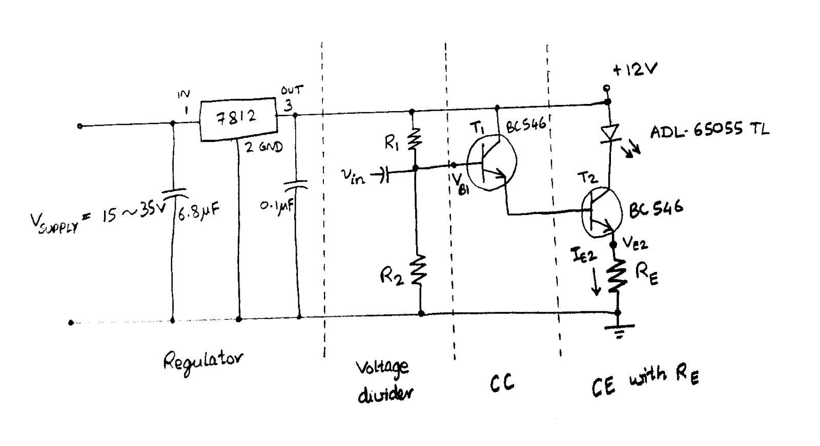
Normally, I use CE with RE configuration as a current source to drive LED as shown in the following figure. In this circuit, laser diode ADL-65055TL from Laser Components was used. Its operating current is 25mA, maximum current is 35mA, and operating voltage is 2.2V.


 For a 12V power supply, assuming VCE(saturation) is approximately zero, RE is calculated as
$$ R_E=\frac{Vcc-V_L}{I_{max}}=\frac{12-2.2}{35m}=280 \Omega $$
I did not want large gain for this CE configuration and bypass capacitor was not used. I wanted the ac output current of this class A amplifier to swing between 23mA and 29 mA. Using the quiescent emitter current for transister 2, IE2=26mA (near operating current), emitter voltage is, VE2=RE x Iop= 280 x 26m = 7.28V. To achieve high input impedance, a CC amplifier was cascaded in front as shown in the following figure.
For a 12V power supply, assuming VCE(saturation) is approximately zero, RE is calculated as
$$ R_E=\frac{Vcc-V_L}{I_{max}}=\frac{12-2.2}{35m}=280 \Omega $$
I did not want large gain for this CE configuration and bypass capacitor was not used. I wanted the ac output current of this class A amplifier to swing between 23mA and 29 mA. Using the quiescent emitter current for transister 2, IE2=26mA (near operating current), emitter voltage is, VE2=RE x Iop= 280 x 26m = 7.28V. To achieve high input impedance, a CC amplifier was cascaded in front as shown in the following figure.

 Assuming base-emitter junction voltage, VBE, as 0.7V, the quiescent base voltage of transister 1 is VB1= 7.28+0.7+0.7=8.68V. Neglecting the small base current, R1 and R2 are calculated as
$$ V_{B1}=Vcc \times \frac{R_2}{R_1+ R_2}$$
$$ \frac{R_1}{R_2}+ 1=\frac{12}{8.68V}$$
Then, R2=2.6 R1. If we choose R1 as 22k arbitrarily, R2 will be 57k. The ac input voltage should be (29-23)m x 280= 1.68V peak to peak. The resulting prototype using available components in my lab is shown here.
Assuming base-emitter junction voltage, VBE, as 0.7V, the quiescent base voltage of transister 1 is VB1= 7.28+0.7+0.7=8.68V. Neglecting the small base current, R1 and R2 are calculated as
$$ V_{B1}=Vcc \times \frac{R_2}{R_1+ R_2}$$
$$ \frac{R_1}{R_2}+ 1=\frac{12}{8.68V}$$
Then, R2=2.6 R1. If we choose R1 as 22k arbitrarily, R2 will be 57k. The ac input voltage should be (29-23)m x 280= 1.68V peak to peak. The resulting prototype using available components in my lab is shown here.




Thursday, July 19, 2012
Myanmar (Burmese) Language with XeTeX and LuaTeX
To properly render Myanmar fonts using LaTeX, it is necessary to use TeX typesetting engines that support Unicode such as XeTeX and LuaTeX. You should make sure that your TeX Live or MiKTeX version is up to date and XeTeX and LuaTeX are bundled with them.
To build TeX files conveniently, you can define user command in editors such as TeXmaker or TeXstudio. In TeXstudio, click Configure TeXstudio... command in the Options menu. Then, go to Commands and copy the command for the PdfLaTeX.
 After that, go to User menu and click User Commands -> Edit User Commands and click green plus sign. Paste the command that you have copied and replace pdflatex with xelatex for XeTeX. Follow the same procedure and use lualatex for LuaTeX.
 The following example TeX file, Z1.tex, works with both xelatex and lualatex.
 XeTeX can render Zawgyi-One and Padauk on all platforms, and Myanmar MN on Mac OS X. Although there is no problem for Zawgyi-One, Unicode fonts such as Padauk require renderer to be defined. In the following example, Renderer=Graphite defines Graphite as the renderer. For Myanmar MN font, the renderer should be explicitly defined as Renderer=AAT. See example XeFontspec.tex as shown below.
 Another way to define renderer instead of using \fontspec[Renderer=Graphite]{Padauk} is
\font\1="Padauk/GR" \1 , where /GR is to explicitly use the Graphite font renderer. Other possible options are /AAT to explicitly use the ATSUI renderer (Mac OS X only) and /ICU to explicitly use the ICU OpenType renderer. However, defining renderer does not works for xelatex versions on my Windows XP and Ubuntu Linux. Fortunately, I found a way at Calmhill's blog that uses \fontspec[Script=Myanmar]{Padauk} to make Padauk works on them. An example is XePadauk.tex.
Another way to define renderer instead of using \fontspec[Renderer=Graphite]{Padauk} is
\font\1="Padauk/GR" \1 , where /GR is to explicitly use the Graphite font renderer. Other possible options are /AAT to explicitly use the ATSUI renderer (Mac OS X only) and /ICU to explicitly use the ICU OpenType renderer. However, defining renderer does not works for xelatex versions on my Windows XP and Ubuntu Linux. Fortunately, I found a way at Calmhill's blog that uses \fontspec[Script=Myanmar]{Padauk} to make Padauk works on them. An example is XePadauk.tex.
 An example for Myanmar MN is XeMyanmarMN.tex. Currently, according to my tests, Myanmar3 does not work on all platforms.
Updated post: A LaTeX Report Template for Myanmar Language Using XeTeX


\documentclass{article}
\usepackage{fontspec}
\setmainfont{Zawgyi-One}
\begin{document}
ျမန္မာစာ
\end{document}
Another example for lualatex that includes lua script is luaZ1.tex. I have tested laulatex with Zawgyi-One, Padauk, Myanmar3, and Myanmar MN. And I found that only Zawgyi-One works with current version (LuaTeX, Version beta-0.70.1-2011082320).


Updated post: A LaTeX Report Template for Myanmar Language Using XeTeX
Subscribe to:
Posts (Atom)