Current Driver for Laser Diode

Normally, I use CE with R_E configuration as a current source to drive LED as shown in the following figure. In this circuit, laser diode ADL-65055TL from Laser Components was used. Its operating current is 25mA, maximum current is 35mA, and operating voltage is 2.2V.

For a 12V power supply, assuming V_{CE(saturation)} is approximately zero, R_E is calculated as $$ R_E=\frac{Vcc-V_L}{I_{max}}=\frac{12-2.2}{35m}=280 \Omega $$ I did not want large gain for this CE configuration and bypass capacitor was not used. I wanted the ac output current of this class A amplifier to swing between 23mA and 29 mA. Using the quiescent emitter current for transister 2, I_E2=26mA (near operating current), emitter voltage is, V_E2=R_E x I_op= 280 x 26m = 7.28V. To achieve high input impedance, a CC amplifier was cascaded in front as shown in the following figure.

Assuming base-emitter junction voltage, V_BE, as 0.7V, the quiescent base voltage of transister 1 is V_B1= 7.28+0.7+0.7=8.68V. Neglecting the small base current, R₁ and R₂ are calculated as $$ V_{B1}=Vcc \times \frac{R_2}{R_1+ R_2}$$ $$ \frac{R_1}{R_2}+ 1=\frac{12}{8.68V}$$ Then, R₂=2.6 R₁. If we choose R₁ as 22k arbitrarily, R₂ will be 57k. The ac input voltage should be (29-23)m x 280= 1.68V peak to peak. The resulting prototype using available components in my lab is shown here.

Myanmar (Burmese) Language with XeTeX and LuaTeX

To properly render Myanmar fonts using LaTeX, it is necessary to use TeX typesetting engines that support Unicode such as XeTeX and LuaTeX. You should make sure that your TeX Live or MiKTeX version is up to date and XeTeX and LuaTeX are bundled with them. To build TeX files conveniently, you can define user command in editors such as TeXmaker or TeXstudio. In TeXstudio, click Configure TeXstudio... command in the Options menu. Then, go to Commands and copy the command for the PdfLaTeX.

After that, go to User menu and click User Commands -> Edit User Commands and click green plus sign. Paste the command that you have copied and replace pdflatex with xelatex for XeTeX. Follow the same procedure and use lualatex for LuaTeX.

The following example TeX file, Z1.tex, works with both xelatex and lualatex.

\documentclass{article}
\usepackage{fontspec}
\setmainfont{Zawgyi-One}
\begin{document}
ျမန္မာစာ
\end{document}

Another example for lualatex that includes lua script is luaZ1.tex. I have tested laulatex with Zawgyi-One, Padauk, Myanmar3, and Myanmar MN. And I found that only Zawgyi-One works with current version (LuaTeX, Version beta-0.70.1-2011082320).

XeTeX can render Zawgyi-One and Padauk on all platforms, and Myanmar MN on Mac OS X. Although there is no problem for Zawgyi-One, Unicode fonts such as Padauk require renderer to be defined. In the following example, Renderer=Graphite defines Graphite as the renderer. For Myanmar MN font, the renderer should be explicitly defined as Renderer=AAT. See example XeFontspec.tex as shown below.

Another way to define renderer instead of using \fontspec[Renderer=Graphite]{Padauk} is \font\1="Padauk/GR" \1 , where /GR is to explicitly use the Graphite font renderer. Other possible options are /AAT to explicitly use the ATSUI renderer (Mac OS X only) and /ICU to explicitly use the ICU OpenType renderer. However, defining renderer does not works for xelatex versions on my Windows XP and Ubuntu Linux. Fortunately, I found a way at Calmhill's blog that uses \fontspec[Script=Myanmar]{Padauk} to make Padauk works on them. An example is XePadauk.tex.

An example for Myanmar MN is XeMyanmarMN.tex. Currently, according to my tests, Myanmar3 does not work on all platforms.

Updated post: A LaTeX Report Template for Myanmar Language Using XeTeX

LaTeX Bibliography with TeXstudio

TeXstudio (formerly TexMakerX, http://texstudio.sourceforge.net/) is an integrated environment for writing LaTeX documents. When you get a paper, there is normally the citation for that paper in BibTeX style. You can save the BibTeX entry for each paper in a BibTeX database file that has .bib file extension. In TeXstudio, it is also easy to create a BibTeX entry yourself. For example, create a new BibTeX database file, Ref1.bib and click bibliography menu. Thereafter, you can choose the command for your paper type. Both the required fields and optional fields will be inserted. If you want to clear the optional fields, you can click the clean command. The easiest way is to use BibTeX insert dialog ... as shown in the following figure.




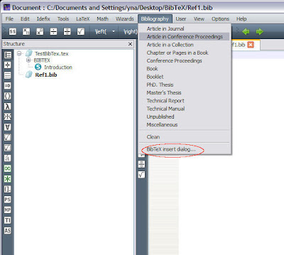
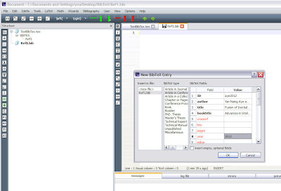
When the new BibTeX entry dialog appears, you can fill the fields you want and click OK. When you filled the author names, they must be separated by the word and. Create a new TeX file, e.g. TestBibTex.tex, and you can use the database as follows. In this example the popular style, ieeetr, is used so that the references will be numbered in order of appearance. The database file, Ref1.bib, that you created is included using \bibliography{Ref1}.





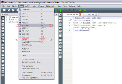
Normally, you need to run LaTeX several times as shown in the following steps to produce the proper output. (you need to have MiKTeX or TeX Live software installed in your computer.) If you use pdflatex, run
Step 1. pdflatex
Step 2. bibtex
Step 3. pdflatex
Step 4. pdflatex
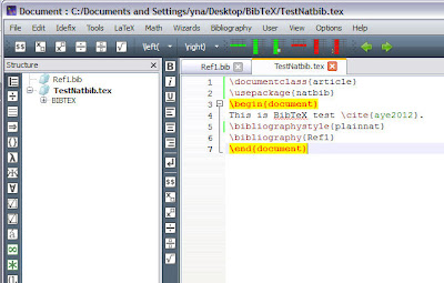
as shown in the following figure. Another good thing about TeXstudio is that you just need to press 'F1' for Quick Build only one time and it will carry out everything to produce the final pdf output. If you want author-year style citation, you can use \usepackage{natbib} as shown in the following figure.



The example files can be downloaded in the following links.
TestBibTex.tex
TestNatbib.tex
Ref1.bib
Using a software for management is more convenient and JabRef Reference Manager is a good one.
Ref: http://en.wikibooks.org/wiki/LaTeX/Bibliography_Management

Skeleton of Image Region

The structural shape of an image region can be represented by a graph. It is achieved by using a thinning algorithm. The resulting graph is called the skeleton of the region. It can be a useful preprocessing step for some applications such as optical character recognition. The following figures shows an original structural shape and its skeleton.

The skeleton of a region is obtained using various methods. Two popular methods among them are Medial Axis Transformation (MAT) , and Two Step Thinning. In Medial Axis Transformation, each point in the region finds its closest neighbour on the boundary of the region. If it finds more than one such neighbour, it belongs to the skeleton of the region. Although MAT is easy to understand, it needs a lot of calculation. We find the distance transform of the region first. The distance transform replaces each pixel value in the region with the distance of the pixel from the nearest neighbour on the boundary of the region. The nearer pixels from the boundary have the lower distance values (lower intensity) and the farther pixels from the boundary have the larger distance values (higher intensity). From the distance values, the local maximums along row or column are searched and defined as pixels in the skeleton. The example MATLAB code for MAT can be seen here (MATeg.m). The original image, the distance transformed image, and the skeleton using MAT are shown in the following figures.

Two Step Thinning algorithm is more efficient and faster than MAT. Two step thinning algorithm iterately delete edge points of a region subject to the constraints that deletion of these points does not remove end points, does not break connectivity, and does not cause excessive erosion of the region. The region points are assumed to have value 1 and background points to have value 0. The method consists of successive passes of two basic steps applied to the given region.

With reference to the 8 neighborhood notation shown in the figure, step 1 flags a contour point p1 for deletion if the following conditions are satisfied: (a) 2 ≤ N(p1) ≤ 6 (b) T(p1) = 1 (c) p2.p4.p6 = 0 (d) p4.p6.p8 = 0 where N(p1) is the number of nonzero neighbors of p1, and T(p1) is the number of 0 to 1 transitions in the ordered sequence p2, p3, ... , p8, p9, p2. In step 2, conditions (a) and (b) remain the same, but conditions (c) and (d) are changed to (c') p2.p4.p8= 0 (d') p2.p6.p8= 0 Step 1 is applied to every border pixel in the binary region under consideration. If one or more of conditions (a)-(d) are violated, the value of the point in question is not changed. If all conditions are satisfied the point is flagged for deletion. However, the point is not deleted until all border points have been processed. This delay prevents changing the structure of the data during execution of the algorithm. After step 1 has been applied to all border points, those that were flagged are deleted (changed to 0). Then step 2 is applied to the resulting data in exactly the same manner as step 1. Thus one iteration of the thinning algorithm consists of (1) applying step 1 to flag border points for deletion; (2) deleting the flagged points; (3) applying step 2 to flag the remaining border points for deletion; and (4) deleting the flagged points. This basic procedure is applied iteratively until no further points are deleted, at which time the algorithm terminates, yielding the skeleton of the region. Condition (c) p2.p4.p6 = 0 and (d) p4.p6.p8 = 0 are satisfied simultaneously by the minimum set of values; (p4 = 0 or p6= 0) or (p2=0 and p8=0). Similarly, conditions (c') and (d') are satisfied simultaneously by the following minimum set of values: (p2=0 or p8=0) or (p4=0 and p6=0). The example MATLAB code for Two Step Thinning algorithm can be seen here (TSTeg.m).

The above codes may be useful to understand the methods and to implement them in other programming languages. In MATLAB, the skeleton of all regions in a binary image is generated via function bwmorph. sk=bwmorph(bwImg,'skel',Inf); The result of the above operation is shown below.

Reference: Rafael C. Gonzalez, Richard E. Woods, Steven L. Eddins, "Digital Image Processing Using MATLAB", Second Edition, Mc Graw Hill (Asia), 2011.