I would like to share a small C++ function to translate and rotate images in 3D space in six degree of freedom (6 DoF).
It also adjusts brightness and contrast. I use OpenCV library to perform some image processing.
Showing posts with label Image processing. Show all posts
Showing posts with label Image processing. Show all posts
Wednesday, November 30, 2022
Friday, September 17, 2021
V4L2 Capturing as Bitmap Image
V4L2 (Video for Linux 2) consists of drivers and API for video capturing on Linux
[1].
In this article, we will discuss about using the library and analysis of video capture example.
There are utilities for controlling media devices on Linux called v4l-utils
[2].
We will explore about using and testing webcam with them also.
Thursday, May 14, 2015
Image Retrieval
This is a MatLab program which receives a test image and find the most similar images in the database.
Friday, August 22, 2014
Batch Processing of Images in GIMP
To perform batch processing of images in GIMP, you can get a plug-in called David's Batch Processor at the link - http://members.ozemail.com.au/~hodsond/dbp.html.
Extract the dbp.exe file and put it at C:\Program Files\GIMP 2\lib\gimp\2.0\plug-ins. Then, open GIMP and click Filters menu -> Batch Process... command. A pop-up windows - David's Batch Processor will appear as shown in the following figure and you can do the batch processing that you want.
Saturday, August 16, 2014
Selective Color Modification
I wanted to change the blue color of the road in the following picture to a green color. I wrote a MatLab program and run it in Octave.
Although I can simply use rgb color model to swap blue and green, I feel like it is too specific. That is why, I used hsv color model to change a hue of a color in a more flexible manner.


Wednesday, March 7, 2012
Skeleton of Image Region
The structural shape of an image region can be represented by a graph. It is achieved by using a thinning algorithm. The resulting graph is called the skeleton of the region. It can be a useful preprocessing step for some applications such as optical character recognition. The following figures shows an original structural shape and its skeleton.

 The skeleton of a region is obtained using various methods. Two popular methods among them are Medial Axis Transformation (MAT) , and Two Step Thinning. In Medial Axis Transformation, each point in the region finds its closest neighbour on the boundary of the region. If it finds more than one such neighbour, it belongs to the skeleton of the region. Although MAT is easy to understand, it needs a lot of calculation. We find the distance transform of the region first. The distance transform replaces each pixel value in the region with the distance of the pixel from the nearest neighbour on the boundary of the region. The nearer pixels from the boundary have the lower distance values (lower intensity) and the farther pixels from the boundary have the larger distance values (higher intensity). From the distance values, the local maximums along row or column are searched and defined as pixels in the skeleton. The example MATLAB code for MAT can be seen here (MATeg.m). The original image, the distance transformed image, and the skeleton using MAT are shown in the following figures.


 Two Step Thinning algorithm is more efficient and faster than MAT. Two step thinning algorithm iterately delete edge points of a region subject to the constraints that deletion of these points does not remove end points, does not break connectivity, and does not cause excessive erosion of the region. The region points are assumed to have value 1 and background points to have value 0. The method consists of successive passes of two basic steps applied to the given region.
 With reference to the 8 neighborhood notation shown in the figure, step 1 flags a contour point p1 for deletion if the following conditions are satisfied:
(a) 2 ≤ N(p1) ≤ 6
(b) T(p1) = 1
(c) p2.p4.p6 = 0
(d) p4.p6.p8 = 0
where N(p1) is the number of nonzero neighbors of p1, and T(p1) is the number of 0 to 1 transitions in the ordered sequence p2, p3, ... , p8, p9, p2.
In step 2, conditions (a) and (b) remain the same, but conditions (c) and (d) are changed to
(c') p2.p4.p8= 0
(d') p2.p6.p8= 0
Step 1 is applied to every border pixel in the binary region under consideration. If one or more of conditions (a)-(d) are violated, the value of the point in question is not changed. If all conditions are satisfied the point is flagged for deletion.
However, the point is not deleted until all border points have been processed. This delay prevents changing the structure of the data during execution of the algorithm. After step 1 has been applied to all border points, those that were flagged are deleted (changed to 0). Then step 2 is applied to the resulting data in exactly the same manner as step 1.
Thus one iteration of the thinning algorithm consists of (1) applying step 1 to flag border points for deletion; (2) deleting the flagged points; (3) applying step 2 to flag the remaining border points for deletion; and (4) deleting the flagged points.
This basic procedure is applied iteratively until no further points are deleted, at which time the algorithm terminates, yielding the skeleton of the region.
Condition (c) p2.p4.p6 = 0 and (d) p4.p6.p8 = 0 are satisfied simultaneously by the minimum set of values; (p4 = 0 or p6= 0) or (p2=0 and p8=0). Similarly, conditions (c') and (d') are satisfied simultaneously by the following minimum set of values: (p2=0 or p8=0) or (p4=0 and p6=0).
The example MATLAB code for Two Step Thinning algorithm can be seen here (TSTeg.m).
With reference to the 8 neighborhood notation shown in the figure, step 1 flags a contour point p1 for deletion if the following conditions are satisfied:
(a) 2 ≤ N(p1) ≤ 6
(b) T(p1) = 1
(c) p2.p4.p6 = 0
(d) p4.p6.p8 = 0
where N(p1) is the number of nonzero neighbors of p1, and T(p1) is the number of 0 to 1 transitions in the ordered sequence p2, p3, ... , p8, p9, p2.
In step 2, conditions (a) and (b) remain the same, but conditions (c) and (d) are changed to
(c') p2.p4.p8= 0
(d') p2.p6.p8= 0
Step 1 is applied to every border pixel in the binary region under consideration. If one or more of conditions (a)-(d) are violated, the value of the point in question is not changed. If all conditions are satisfied the point is flagged for deletion.
However, the point is not deleted until all border points have been processed. This delay prevents changing the structure of the data during execution of the algorithm. After step 1 has been applied to all border points, those that were flagged are deleted (changed to 0). Then step 2 is applied to the resulting data in exactly the same manner as step 1.
Thus one iteration of the thinning algorithm consists of (1) applying step 1 to flag border points for deletion; (2) deleting the flagged points; (3) applying step 2 to flag the remaining border points for deletion; and (4) deleting the flagged points.
This basic procedure is applied iteratively until no further points are deleted, at which time the algorithm terminates, yielding the skeleton of the region.
Condition (c) p2.p4.p6 = 0 and (d) p4.p6.p8 = 0 are satisfied simultaneously by the minimum set of values; (p4 = 0 or p6= 0) or (p2=0 and p8=0). Similarly, conditions (c') and (d') are satisfied simultaneously by the following minimum set of values: (p2=0 or p8=0) or (p4=0 and p6=0).
The example MATLAB code for Two Step Thinning algorithm can be seen here (TSTeg.m).
 The above codes may be useful to understand the methods and to implement them in other programming languages. In MATLAB, the skeleton of all regions in a binary image is generated via function bwmorph.
sk=bwmorph(bwImg,'skel',Inf);
The result of the above operation is shown below.
The above codes may be useful to understand the methods and to implement them in other programming languages. In MATLAB, the skeleton of all regions in a binary image is generated via function bwmorph.
sk=bwmorph(bwImg,'skel',Inf);
The result of the above operation is shown below.

Reference: Rafael C. Gonzalez, Richard E. Woods, Steven L. Eddins, "Digital Image Processing Using MATLAB", Second Edition, Mc Graw Hill (Asia), 2011.


Reference: Rafael C. Gonzalez, Richard E. Woods, Steven L. Eddins, "Digital Image Processing Using MATLAB", Second Edition, Mc Graw Hill (Asia), 2011.
Friday, December 16, 2011
Geometric Template Matching in LabVIEW
In NI's IMAQ Vision Concepts Manual, geometric template matching is described as follows.
Geometric matching locates regions in a grayscale image that match a model, or template, of a reference pattern. Geometric matching is specialized to locate templates that are characterized by distinct geometric or shape information.
When using geometric matching, a template is created that represents the object to be searched. Machine vision application then searches for instances of the template in each inspection image and calculates a score for each match. The score relates how closely the template resembles the located matches.
Geometric matching finds template matches regardless of lighting variation, blur, noise, occlusion, and geometric transformations such as shifting, rotation, or scaling of the template.
The VIs such as IMAQ Find CoordSys (Pattern) 2 are used to locate the model. The template for the model is created as discussed in the following steps. Open Template Editor in Windows by clicking Start -> All Programs -> National Instruments -> Vision -> Template Editor.
Click File menu->New Template....
Select Geometric Matching Template (Edge Based) and browse an image to extract the template from.
In the Select Template Region tab, define a region. For example, start at (200,300) and drag the mouse cursor to (232,332) and release it. Then, you can move the selection to the desired location.
In the Define curves tab, specify curve parameters, e.g., Extraction mode to normal, Edge Threshold to 32, Edge Filter size to Fine, Minimum Length to 5, Row Search Step Size to 1 and Column Search Step size to 1. The setting in Customize Scoring and Specify Match Options tabs are set as default.
Save the template by clicking File -> Save Template....
Open Template Editor in Windows by clicking Start -> All Programs -> National Instruments -> Vision -> Template Editor.
Click File menu->New Template....
Select Geometric Matching Template (Edge Based) and browse an image to extract the template from.
In the Select Template Region tab, define a region. For example, start at (200,300) and drag the mouse cursor to (232,332) and release it. Then, you can move the selection to the desired location.
In the Define curves tab, specify curve parameters, e.g., Extraction mode to normal, Edge Threshold to 32, Edge Filter size to Fine, Minimum Length to 5, Row Search Step Size to 1 and Column Search Step size to 1. The setting in Customize Scoring and Specify Match Options tabs are set as default.
Save the template by clicking File -> Save Template....
 As an example, I have created a few VIs at the following link.
Geometric Template Matching on GitHub
Initialization for the VI inputs is shown below.
The VIs such as IMAQ Find CoordSys (Pattern) 2 are used to locate the model. The template for the model is created as discussed in the following steps.


Geometric Template Matching on GitHub
Initialization for the VI inputs is shown below.

Thursday, April 10, 2008
Reverse Macro Ring
Macro lens for close up photos are expensive for me. There are some cheap converter lens, but I don't like to use them after trying a few shots. Later, I found a link about home-made reverse ring here. The followings are about my home made reverse ring. I didn't have an old filter. Therefore, I bought the cheapest body cover ( 5 SGD) and filter (10 SGD).
 Then, I made a hole in the Body Cap. Filter was a new one and it was OK to leave as it was. But I thought it was better to remove the glass and I broke it using a hammer. To prevent the scattering of glass debris, you should pack it with a paper or a plastic or stick it with a piece of tape before you break it.

After putting them together, it became as shown. Take care, to put the thread outside. They must be glued at the sides that has no thread.

 Lens can be fastened in reverse now. The smaller the mm, the bigger the magnification. You can push the aperture lever to get a bigger aperture. I think 50 mm prime lens may be the best to use with reverse ring.

Here are a few shots I tried with this reverse ring.


 Then, I made a hole in the Body Cap. Filter was a new one and it was OK to leave as it was. But I thought it was better to remove the glass and I broke it using a hammer. To prevent the scattering of glass debris, you should pack it with a paper or a plastic or stick it with a piece of tape before you break it.
After putting them together, it became as shown. Take care, to put the thread outside. They must be glued at the sides that has no thread.

 Lens can be fastened in reverse now. The smaller the mm, the bigger the magnification. You can push the aperture lever to get a bigger aperture. I think 50 mm prime lens may be the best to use with reverse ring.
Here are a few shots I tried with this reverse ring.


Sunday, April 6, 2008
HDR in GIMP
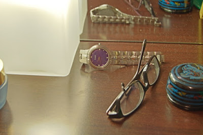
In an HDR (High Dynamic Range) photo, some parts of the photo are too bright and some parts are too dark so that all of them cannot be captured by a camera in a single exposure or cannot be displayed on a screen.
In the following picture, the side of the lamp is too bright and the side of the lacquered box is too dark.
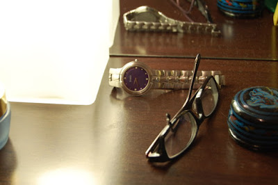 If you increase the exposure, the lacquered box side will be OK. But the lamp side will be too bright.
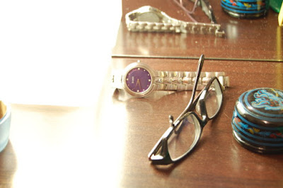 If you decrease the exposure, the lamp side will be just nice and the lacquered box side will be too dark to see properly.

We will use exposure bracketing to solve this problem. Take three exposures, one with normal exposure, another with +2 EV overexposed and the last one with -2EV underexposed. It is better to use a tripod and manual focus mode. Use fixed aperture to get same Depth of Field. After that, you need to put Exposure Blending Plug-in for GIMP.
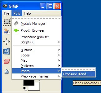
You can download the plug-in from http://turtle.as.arizona.edu/jdsmith/exposure-blend-tinyscheme.scm. For GIMP 2.4.5, you need to put the file into C:\Program Files\GIMP-2.0\share\gimp\2.0\scripts. It can be vary according to your installed location. Then, open GIMP and click Xtns menu -> Photo -> Exposure Blend ... .
 Insert the three pictures there.
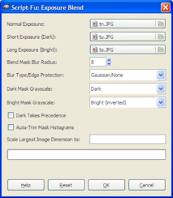 You can use your preferred settings.Click OK. After that you will get an Exposure Blended picture.
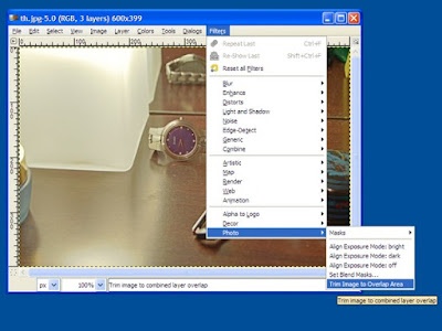
 If your pictures are not exactly the same, there is an auto align feature in some software such as Photoshop, PhotoMatix, etc. However, you need to align manually in GIMP. Go to Filters menu -> Photo -> Align Exposure Mode and you can adjust the layers using difference mode.
 You can also go to layer windows and adjust opacity, layer mask and many others fine tunings of dark layer and bright layer.

Reference:
http://turtle.as.arizona.edu/jdsmith/exposure_blend.php
 If you increase the exposure, the lacquered box side will be OK. But the lamp side will be too bright.
 If you decrease the exposure, the lamp side will be just nice and the lacquered box side will be too dark to see properly.
We will use exposure bracketing to solve this problem. Take three exposures, one with normal exposure, another with +2 EV overexposed and the last one with -2EV underexposed. It is better to use a tripod and manual focus mode. Use fixed aperture to get same Depth of Field. After that, you need to put Exposure Blending Plug-in for GIMP.
You can download the plug-in from http://turtle.as.arizona.edu/jdsmith/exposure-blend-tinyscheme.scm. For GIMP 2.4.5, you need to put the file into C:\Program Files\GIMP-2.0\share\gimp\2.0\scripts. It can be vary according to your installed location. Then, open GIMP and click Xtns menu -> Photo -> Exposure Blend ... .
 Insert the three pictures there.
  You can use your preferred settings.Click OK. After that you will get an Exposure Blended picture.
 If your pictures are not exactly the same, there is an auto align feature in some software such as Photoshop, PhotoMatix, etc. However, you need to align manually in GIMP. Go to Filters menu -> Photo -> Align Exposure Mode and you can adjust the layers using difference mode.
 You can also go to layer windows and adjust opacity, layer mask and many others fine tunings of dark layer and bright layer.
Reference:
http://turtle.as.arizona.edu/jdsmith/exposure_blend.php
Tuesday, March 25, 2008
Velvia
Just a try to get vivid colors something like Fujifilm's Velvia film using free software GIMP. Although you can use Hue-Saturation tool to increase color saturation, the following method is closer to Velvia. Another reason is that Saturation can sometimes posterize color.
Open the picture you want to edit. Open Colors menu -> Compoments -> Channel mixer....
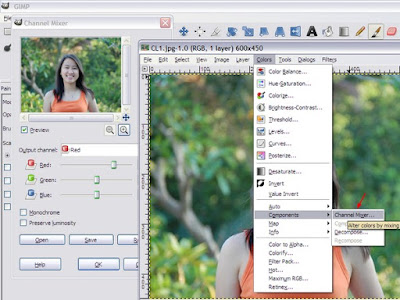 Choose Red in Output Channel and increase Red slider to 150. Reduce Green and Blue sliders to -25 to balance it. Repeat the similar steps for Green and Blue channels.
Click OK. Then choose Colors menu->Levels and increase the slider below input levels until you get a desire contrast.
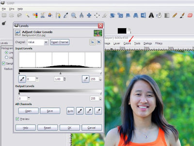 After that, you will get a Velvia style photo. See the following pictures as a comparison between original and Velvia style.
Before
 After
After

Reference:
http://photoshoptutorials.ws/photoshop-tutorials/photo-effects/velvia.html
 Choose Red in Output Channel and increase Red slider to 150. Reduce Green and Blue sliders to -25 to balance it. Repeat the similar steps for Green and Blue channels.
Output Channel: Red
Red: +150
Green: -25
Blue: -25

Output Channel: Green
Red: -25
Green: +150
Blue: -25

Output Channel: Blue
Red: -25
Green: -25
Blue: +150
Click OK. Then choose Colors menu->Levels and increase the slider below input levels until you get a desire contrast.
 After that, you will get a Velvia style photo. See the following pictures as a comparison between original and Velvia style.
Before
 After
After
Reference:
http://photoshoptutorials.ws/photoshop-tutorials/photo-effects/velvia.html
Lomography
Getting a photo using GIMP that is similar to the one taken with Lomo Lens is discussed. You can read about Lomography here. Lomo photos have distinct vignette -darken edges- caused by the lens. First, we will try to mimic it in our picture. Choose circle selection tool from GIMP tool box. Select the whole picture. Click Select Menu-> Invert.

Choose Layer Menu-> New layer (or) press Ctrl+Shift+N. Then give a layer name something like Vignette. Choose Transparency and click OK.

As shown in the following picture, choose black for Foreground color and white for Background color. Select "Vignette" layer and go to Dialog menu->layer-> layer dialog. Then fill black color using Edit menu-> Fill with FG color. Remove selection by clicking select menu->None.

Open Filter menu->Blur->Gaussian Blur. Set the blur radius to about one quarter of the width of photo. In this case, set it to 150 and click OK.

Go to Layer dialog and set the Opacity of Vignette layer to about 75%. In fact, the value can be set according to your preferences.

Select the Background layer. Open Dialog menu->Channels->Channels dialog. Select Red channel.

Open Color menu->Brightness-Contrast and increase Contrast about 50.

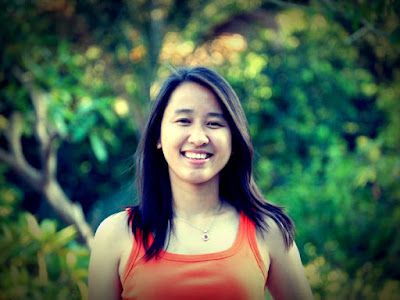
Similarly, increase contrast to 50 for Green channel. After that, you will get a lomo style photo. See the following photos for a comparison between original and lomo style photos.
Before
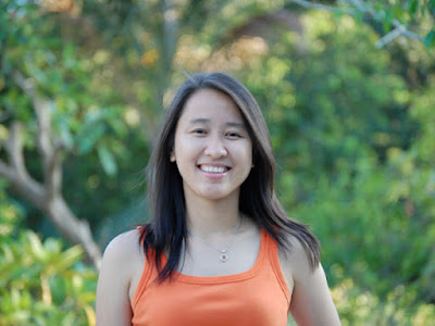
After
Reference:
http://photoshoptutorials.ws/photoshop-tutorials/photo-effects/lomography.html

Choose Layer Menu-> New layer (or) press Ctrl+Shift+N. Then give a layer name something like Vignette. Choose Transparency and click OK.

As shown in the following picture, choose black for Foreground color and white for Background color. Select "Vignette" layer and go to Dialog menu->layer-> layer dialog. Then fill black color using Edit menu-> Fill with FG color. Remove selection by clicking select menu->None.

Open Filter menu->Blur->Gaussian Blur. Set the blur radius to about one quarter of the width of photo. In this case, set it to 150 and click OK.

Go to Layer dialog and set the Opacity of Vignette layer to about 75%. In fact, the value can be set according to your preferences.

Select the Background layer. Open Dialog menu->Channels->Channels dialog. Select Red channel.

Open Color menu->Brightness-Contrast and increase Contrast about 50.

Similarly, increase contrast to 50 for Green channel. After that, you will get a lomo style photo. See the following photos for a comparison between original and lomo style photos.
Before

After

Reference:
http://photoshoptutorials.ws/photoshop-tutorials/photo-effects/lomography.html
Subscribe to:
Posts (Atom)