Monday, January 21, 2013

k-means clustering using custom distance measuring method

I have developed a MATLAB function to perform k-means clustering which enables custom distance measuring method. For example, to sort out histograms, chi-square distance may be more suitable. The following example function uses chi-square distance and you can replace it with any distance measurement method.

%k-means test program
X = [randn(100,2)+ones(100,2);...
     randn(100,2)-ones(100,2)];

[idx,ctrs] = KMeansCustom(X,2);
%[idx,ctrs] = kmeans(X,2);

plot(X(idx==1,1),X(idx==1,2),'r.','MarkerSize',12)
hold on
plot(X(idx==2,1),X(idx==2,2),'b.','MarkerSize',12)
plot(ctrs(:,1),ctrs(:,2),'kx',...
     'MarkerSize',12,'LineWidth',2)
legend('Cluster 1','Cluster 2','Centroids',...
       'Location','NW')

function [Idx,C]=KMeansCustom(X,k)
%KMeansCustom partitions the points in the n-by-d data matrix X into k clusters.
%[Idx,C]= KMeansCustom(X,k) returns 
%n-by-1 vector IDX containing the cluster indices of each point and 
%k-by-d matrix C containing the k cluster centroid locations.
%For n sample points with d dimensions in each point, X has n rows and d columns.
%File name: KMeanCustom.m
%Author: Yan Naing Aye
%Website: http://cool-emerald.blogspot.sg/


%%%%%%%%%%%%%%%%%%%%%%%%%%%%%%%%%%%%%%%%%%%%%%%%%%%%%%%%%%%
%Define maximum number of iterations
MaxIter=500;
%%%%%%%%%%%%%%%%%%%%%%%%%%%%%%%%%%%%%%%%%%%%%%%%%%%%%%%%%%%
[n,d]=size(X);
k=round(k);
%%%%%%%%%%%%%%%%%%%%%%%%%%%%%%%%%%%%%%%%%%%%%%%%%%%%%%%%%%%
%step1 :arbitrarily choose k samples as the initial cluster centers
p=randperm(n);
Mu=X(p(1:k),:);
D=zeros(k,d);
for t=1:MaxIter
 %step2:distribute the samples X  to the clusters 
 for j=1:k
        for i=1:n
            D(j,i)=ChiDist(X(i,:),Mu(j,:));%Use custom distance
        end
 end
 [ValMin,IndexMin]=min(D);
 %%%%%%%%%%%%%%%%%%%%%%%%%%%%%%%%%%%%%%%%%%%%%%%%%%%%%%%%%%%
 %step 3: update the cluster centers
    OldMu=Mu;
 for i=1:k
        Mu(i,:)=mean(X(IndexMin==i,:));
 end
 %%%%%%%%%%%%%%%%%%%%%%%%%%%%%%%%%%%%%%%%%%%%%%%%%%%%%%%%%%%%%
 %step4 :check convergence
 if sum(sum(abs(OldMu-Mu))) == 0 %< 1e-9
        break
 end
end
Idx=IndexMin';
C=Mu;

function d=ChiDist(v1,v2)
    dv=(v1-v2).^2;
    sv=abs(v1)+abs(v2);
    %------------------------------------------------------
    %eliminate zero denominator
    sv(sv==0)=1e-9;
    %------------------------------------------------------
    d=sum(dv./sv)./2;    
end

Amplitude spectrum of a signal using Fourier transform

I have developed a MATLAB function to calculate amplitude spectrum of a signal using Fourier transform. Example usage of the function and implementation is shown below. Another example MATLAB program using built in function fft is also demonstrated. I hope they will be helpful for those who want to find amplitude spectrum or power spectrum of a signal.

%Example MATLAB code to test function FX
Fs=100;
t=(0:1/Fs:1-1/Fs)';
x=2*cos(2*pi*5*t)+sin(2*pi*10*t);
[f a]=FX(x,Fs);
plot(f,a);

function [f a]=FX(x,fs)
%Calculates amplitude spectrum of a signal x using Fourier transform
%[f a]=FX(x,fs)
%Input: x=signal, fs = sampling rate
%Output: f = frequency axis, a = amplitude spectrum
%File name: FX.m
%Author: Yan Naing Aye
%Website: http://cool-emerald.blogspot.sg/

dT = 1/fs; 
N=length(x);
dF=1/(N*dT);
NF=fs/2;%Nyquist Freq
%You can always limit freq range for faster performance
%NF=20;
t=(0:dT:(N-1)*dT)';
f=(0:dF:NF)';
a=f;%initialize a
a(1)=mean(x);
for i=2 : length(a)
    b=(2*mean(x.*cos(2*pi*dF*(i-1)*t)));
    c=(2*mean(x.*sin(2*pi*dF*(i-1)*t)));
    a(i)=sqrt(b^2+c^2);
end

%MATLAB program to calculates amplitude spectrum of a signal x using fft
%Author: Yan Naing Aye
%Website: http://cool-emerald.blogspot.sg/

Fs=100;
t=(0:1/Fs:1-1/Fs)';
x=2*cos(2*pi*5*t)+sin(2*pi*10*t);
L=length(x);

A=2*abs(fft(x)/L);
A=A(1:Fs/2+1);
f = Fs/2*linspace(0,1,Fs/2+1);
plot(f,A);

Sunday, January 13, 2013

Changing sampling rate using quadratic regression

I want to change sampling rate of a signal from 333Hz to 5000Hz. To get a smoother result, I have implemented second order hold system instead of popular zero order hold (ZOH) system. This approach can also be used for down sampling. Another possible application is to filter out noise without introducing phase delay. And it can be useful for real-time application.

Approach 1: Quadratic regression
Quadratic function is defined as

$$f=w_0+w_1 x + w_2 x^2$$

Then, cost function to be minimized is defined as

$$J(w)=\frac{1}{2}\sum_{i=1}^{n}(y_i-f_i)^2$$
$$J(w)=\frac{1}{2}\sum_{i=1}^{n}(y_i-w_0+w_1 x_i + w_2 x_i^2)^2$$

Optimal weights can be found by differentiating the cost function and setting them to zero.

$$\frac{\partial J(w)}{\partial w_0}=0$$
$$-\sum_{i=1}^{n}(y_i-w_0+w_1 x_i + w_2 x_i^2)=0$$
$$w_0\sum_{i=1}^{n}1+w_1\sum_{i=1}^{n}x_i+w_2\sum_{i=1}^{n}x_i^2=\sum_{i=1}^{n}y_i$$

Similarly, differentiating with w1 and w2 gives,

$$w_0\sum_{i=1}^{n}x_i+w_1\sum_{i=1}^{n}x_i^2+w_2\sum_{i=1}^{n}x_i^3=\sum_{i=1}^{n}y_i x_i$$
$$w_0\sum_{i=1}^{n}x_i^2+w_1\sum_{i=1}^{n}x_i^3+w_2\sum_{i=1}^{n}x_i^4=\sum_{i=1}^{n}y_i x_i^2$$

When these three equations are written in matrix form.

$$ \begin{bmatrix} \sum_{i=1}^{n}1 & \sum_{i=1}^{n}x_i & \sum_{i=1}^{n}x_i^2 \\ \sum_{i=1}^{n}x_i & \sum_{i=1}^{n}x_i^2 & \sum_{i=1}^{n}x_i^3 \\ \sum_{i=1}^{n}x_i^2 & \sum_{i=1}^{n}x_i^3 & \sum_{i=1}^{n}x_i^4 \end{bmatrix} \begin{bmatrix} w_0 \\ w_1 \\ w_2 \end{bmatrix} = \begin{bmatrix} \sum_{i=1}^{n}y_i \\ \sum_{i=1}^{n}y_i x_i \\ \sum_{i=1}^{n}y_i x_i^2 \end{bmatrix} $$
$$\mathbf{A}\mathbf{W}=\mathbf{B}$$
$$\mathbf{W}=\mathbf{A}^{-1}\mathbf{B}$$

Approach 2: Three equations
In our case, we can use only the last three points and we can get three equations from these three points.


$$y_1=w_0+w_1 x_1 + w_2 x_1^2$$
$$y_2=w_0+w_1 x_2 + w_2 x_2^2$$
$$y_3=w_0+w_1 x_3 + w_2 x_3^2$$
$$ \begin{bmatrix} 1 & x_1 & x_1^2 \\ 1 & x_2 & x_2^2 \\ 1 & x_3 & x_3^2 \end{bmatrix} \begin{bmatrix} w_0 \\ w_1 \\ w_2 \end{bmatrix} = \begin{bmatrix} y_1 \\ y_2 \\ y_3 \end{bmatrix} $$
$$\mathbf{A}\mathbf{W}=\mathbf{B}$$
$$\mathbf{W}=\mathbf{A}^{-1}\mathbf{B}$$

Approach 3: Two equations
If we define x1=-1, x2=0, and x3=1, y2 is equal to w0. And,

$$y_1=y_2-w_1+ w_2$$
$$y_3=y_2+w_1+ w_2$$
$$ \begin{bmatrix} -1 & 1 \\ 1 & 1 \end{bmatrix} \begin{bmatrix} w_1 \\ w_2 \end{bmatrix} = \begin{bmatrix} y_1-y_2 \\ y_3-y2 \end{bmatrix} $$
$$ \begin{bmatrix} w_1 \\ w_2 \end{bmatrix} = \begin{bmatrix} -0.5 & 0.5 \\ 0.5 & 0.5 \end{bmatrix} \begin{bmatrix} y_1-y_2 \\ y_3-y2 \end{bmatrix} $$

Then, we have

$$w_0=y_2$$
$$w_1=-0.5(y_1-y_2)+0.5(y_3-y2)$$
$$w_2=0.5(y_1-y_2)+0.5(y_3-y2)$$

I have tested the above three approaches using MatLab and it is shown below.
%-------------------------------------------------------------------------
clc;
close all;
clear all;
%-------------------------------------------------------------------------
% y= w0 + w1*x + w2* x^2;
%-------------------------------------------------------------------------
%Got x and y
x=[-1 0 1]';
Wo=[4 3 2]';
y=Wo(1)+Wo(2)*x+Wo(3).*x.*x;

%-------------------------------------------------------------------------
%Approach 1
%Polynomial regression of order 2
%For n=3
S1=3;
Sx=sum(x);
Sx2=sum(x.*x);
Sx3=sum(x.*x.*x);
Sx4=sum(x.*x.*x.*x);
Sy=sum(y);
Syx=sum(y.*x);
Syx2=sum(y.*x.*x);

P=[S1 Sx Sx2; Sx Sx2 Sx3; Sx2 Sx3 Sx4];
B=[Sy Syx Syx2]';
%P1=P^(-1);
W1=P\B

%-------------------------------------------------------------------------
%Approach 2
%Linear equations
A=[1 x(1) x(1)*x(1);1 x(2) x(2)*x(2); 1 x(3) x(3)*x(3)];
W2=A\y
%-------------------------------------------------------------------------
%Approach 3
%Only 2 linear equations
w0=y(2);
w1=-0.5*( y(1)- y(2))+0.5*( y(3)- y(2));
w2=0.5*( y(1)- y(2))+0.5*(y(3)- y(2));
W3=[w0 w1 w2]'
%-------------------------------------------------------------------------
The following figure shows the result of using this method (blue color plot) compare to ordinary zero order hold (black color plot). This method gives much more smoother result but it should be noted that it introduces one sample delay.
The implementation of this method in LabVIEW using C code is shown in the following figure.
The first two approaches involve finding inverse of a 3x3 matrix and I have developed a C program as shown below.
#include
#include
main()
{
    float M[3][3]={{3,0,2},{0,2,0},{2,0,2}}; //initialize a 3x3 matrix
    float N[3][3]={{0,0,0},{0,0,0},{0,0,0}}; //allocate for inverse
    int i,j;
    float d;
    //-------------------------------------------------------------------------
    N[0][0]=(M[1][1]*M[2][2]-M[2][1]*M[1][2]);
    N[1][0]=-(M[1][0]*M[2][2]-M[2][0]*M[1][2]);
    N[2][0]=(M[1][0]*M[2][1]-M[1][1]*M[2][0]);
    d=M[0][0]*N[0][0]+M[0][1]*N[1][0]+M[0][2]*N[2][0];
    N[0][0]/=d;
    N[1][0]/=d;
    N[2][0]/=d;
    N[0][1]=-(M[0][1]*M[2][2]-M[0][2]*M[2][1])/d;
    N[1][1]=(M[0][0]*M[2][2]-M[0][2]*M[2][0])/d;
    N[2][1]=-(M[0][0]*M[2][1]-M[0][1]*M[2][0])/d;
    N[0][2]=(M[0][1]*M[1][2]-M[0][2]*M[1][1])/d;
    N[1][2]=-(M[0][0]*M[1][2]-M[0][2]*M[1][0])/d;
    N[2][2]=(M[0][0]*M[1][1]-M[0][1]*M[1][0])/d;
    //-------------------------------------------------------------------------
    //print 3x3 matrix
    for(i=0;i<3;i++)
    {
        for(j=0;j<3;j++) printf("%3.4f ",N[i][j]);
        printf("\n");
    }
    getch();
    return 0;
}

Wednesday, January 9, 2013

Rotations in 3D space using Euler angles

Rotations in 3D space to relate body reference frame of a device to world reference frame using an Euler angle sequence are discussed. Euler stated that

Any two independent orthonormal coordinate frames can be related by a sequence of rotations (not more than three) about coordinate axes, where no two successive rotations may be about the same axis.
The illustration of the world reference frame, {M}, and the body reference frame, {B}, is shown in the following figure.

Pan angle rotation, α, is acquired using computer vision. And, tilt angle rotation, β, and roll angle rotation, γ, are acquired by sensing the gravity, g, using onboard accelerometers. Let us consider the roll angle first, assuming there are no pan and tilt angles. When the roll angle, γ, is zero Y-axis is upward vertical and X-axis is horizontal pointing according to right handed rule. The gravity sensed by X-axis accelerometer and Y-axis accelerometer are denoted by gx and gy respectively. The definition of the roll angle is illustrated in the following figure.
The roll angle, γ, is calculated as

$$ \gamma = \tan^{-1}\frac{gx}{gy} $$.

Then, it is checked for second and third quadrants as
if(gy<0)
  if(gx>=0)
    γ=π+γ;
  else
    γ=-π+γ;
  end
end
The roll angle rotation matrix, Rγ, is obtained as follows.

$$ \mathbf{R}_{\gamma}= \begin{bmatrix} \cos(\gamma) & -\sin(\gamma) & 0 \\ \sin(\gamma) & \cos(\gamma) & 0 \\ 0 & 0 & 1 \end{bmatrix}$$

After the roll angle is corrected, let us consider for tilt angle. The definition of the tilt angle is illustrated in the following figure.
The tilt angle, β, can be calculated from Y and Z components of the gravity. It is important to note that these gravity component values should be in the roll angle rotated frame. The new values for the gravity components are obtained as

$$ \begin{bmatrix} gx2 \\ gy2 \\ gz2 \end{bmatrix} = \mathbf{R}_{\gamma} \begin{bmatrix} gx \\ gy \\ gz \end{bmatrix} $$

The tilt angle, β, is calculated as
$$\beta = \tan^{-1}\frac{gy2}{gz2} $$.
Then, it is checked for second and third quadrants as
if(gz2>=0)
  if(gy2>=0)
    β=-π+β;
  else
    β=π+β;
  end
end
The tilt angle rotation matrix, Rβ, is obtained as follows.

$$ \mathbf{R}_{\beta}= \begin{bmatrix} 1 & 0 & 0\\ 0 & \cos(\gamma) & -\sin(\gamma) \\ 0 & \sin(\gamma) & \cos(\gamma) \end{bmatrix}$$

Similarly, calculation of the pan angle rotation matrix, Rα, and description of pan angle definition are as follows.

$$ \mathbf{R}_{\alpha}= \begin{bmatrix} \cos(\alpha) & -\sin(\alpha) & 0 \\ \sin(\alpha) & \cos(\alpha) & 0 \\ 0 & 0 & 1 \end{bmatrix}$$

The product of rotation matrices is itself a rotation matrix. $$ \mathbf{R}=\mathbf{R}_{\alpha} \mathbf{R}_{\beta} \mathbf{R}_{\gamma}$$
And, M=RB
Since R is a rotation matrix, inverse of R is obtained by transposing R. The implementation of this 3D rotation in LabVIEW using MabLab code is shown in the following figure.

Quaternion algebra is also easy and popular approach for such 3D transformation.

Reference:
Kuipers, Jack B., Quaternions and rotation sequences : a primer with applications to orbits, aerospace, and virtual reality, Princeton University Press, 1999, ISBN: 0691058725.

Wednesday, December 19, 2012

Current Driver for Laser Diode

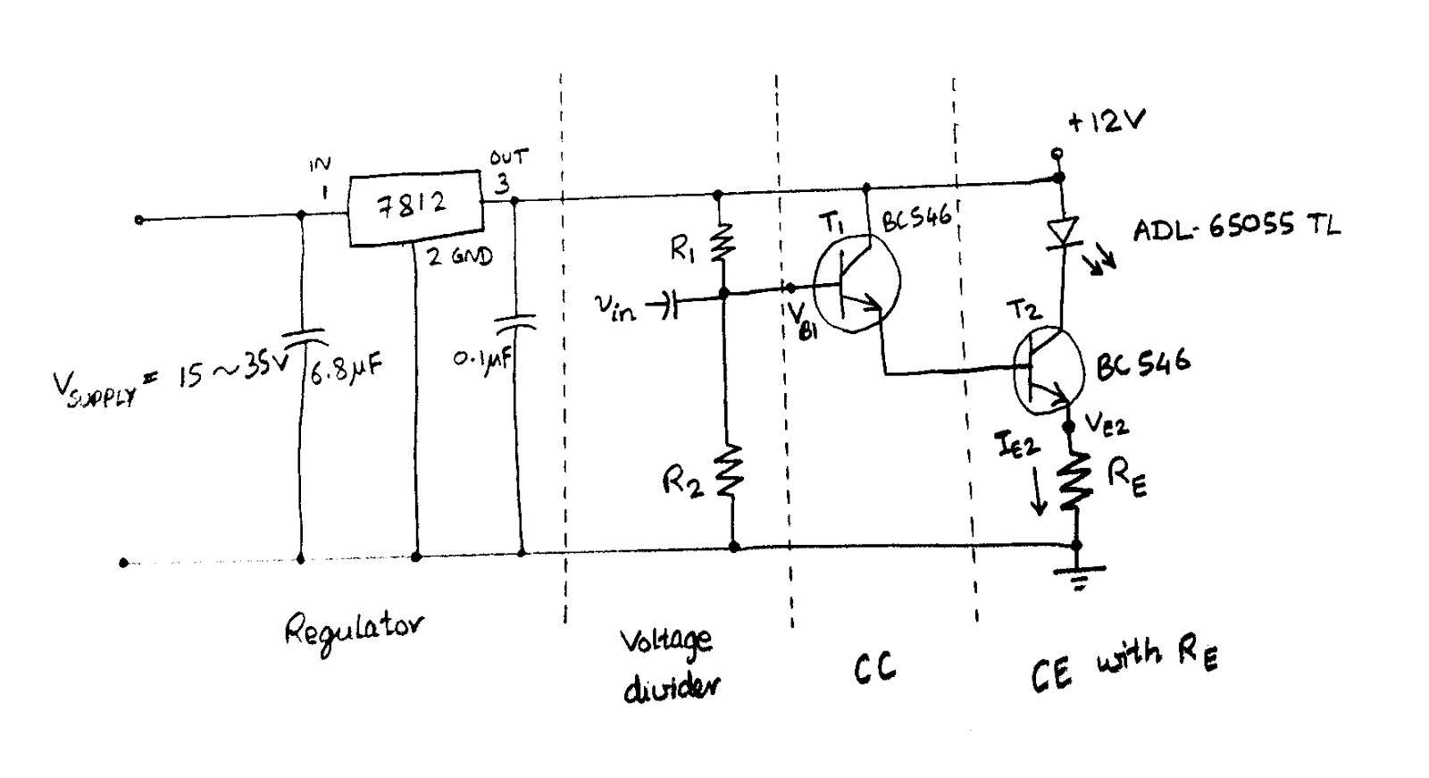
Normally, I use CE with RE configuration as a current source to drive LED as shown in the following figure. In this circuit, laser diode ADL-65055TL from Laser Components was used. Its operating current is 25mA, maximum current is 35mA, and operating voltage is 2.2V.
For a 12V power supply, assuming VCE(saturation) is approximately zero, RE is calculated as $$ R_E=\frac{Vcc-V_L}{I_{max}}=\frac{12-2.2}{35m}=280 \Omega $$ I did not want large gain for this CE configuration and bypass capacitor was not used. I wanted the ac output current of this class A amplifier to swing between 23mA and 29 mA. Using the quiescent emitter current for transister 2, IE2=26mA (near operating current), emitter voltage is, VE2=RE x Iop= 280 x 26m = 7.28V. To achieve high input impedance, a CC amplifier was cascaded in front as shown in the following figure.
Assuming base-emitter junction voltage, VBE, as 0.7V, the quiescent base voltage of transister 1 is VB1= 7.28+0.7+0.7=8.68V. Neglecting the small base current, R1 and R2 are calculated as $$ V_{B1}=Vcc \times \frac{R_2}{R_1+ R_2}$$ $$ \frac{R_1}{R_2}+ 1=\frac{12}{8.68V}$$ Then, R2=2.6 R1. If we choose R1 as 22k arbitrarily, R2 will be 57k. The ac input voltage should be (29-23)m x 280= 1.68V peak to peak. The resulting prototype using available components in my lab is shown here.

Thursday, July 19, 2012

Myanmar (Burmese) Language with XeTeX and LuaTeX

To properly render Myanmar fonts using LaTeX, it is necessary to use TeX typesetting engines that support Unicode such as XeTeX and LuaTeX. You should make sure that your TeX Live or MiKTeX version is up to date and XeTeX and LuaTeX are bundled with them. To build TeX files conveniently, you can define user command in editors such as TeXmaker or TeXstudio. In TeXstudio, click Configure TeXstudio... command in the Options menu. Then, go to Commands and copy the command for the PdfLaTeX.
After that, go to User menu and click User Commands -> Edit User Commands and click green plus sign. Paste the command that you have copied and replace pdflatex with xelatex for XeTeX. Follow the same procedure and use lualatex for LuaTeX.
The following example TeX file, Z1.tex, works with both xelatex and lualatex.
\documentclass{article}
\usepackage{fontspec}
\setmainfont{Zawgyi-One}
\begin{document}
ျမန္မာစာ
\end{document}
Another example for lualatex that includes lua script is luaZ1.tex. I have tested laulatex with Zawgyi-One, Padauk, Myanmar3, and Myanmar MN. And I found that only Zawgyi-One works with current version (LuaTeX, Version beta-0.70.1-2011082320).
XeTeX can render Zawgyi-One and Padauk on all platforms, and Myanmar MN on Mac OS X. Although there is no problem for Zawgyi-One, Unicode fonts such as Padauk require renderer to be defined. In the following example, Renderer=Graphite defines Graphite as the renderer. For Myanmar MN font, the renderer should be explicitly defined as Renderer=AAT. See example XeFontspec.tex as shown below.
Another way to define renderer instead of using \fontspec[Renderer=Graphite]{Padauk} is \font\1="Padauk/GR" \1 , where /GR is to explicitly use the Graphite font renderer. Other possible options are /AAT to explicitly use the ATSUI renderer (Mac OS X only) and /ICU to explicitly use the ICU OpenType renderer. However, defining renderer does not works for xelatex versions on my Windows XP and Ubuntu Linux. Fortunately, I found a way at Calmhill's blog that uses \fontspec[Script=Myanmar]{Padauk} to make Padauk works on them. An example is XePadauk.tex.
An example for Myanmar MN is XeMyanmarMN.tex. Currently, according to my tests, Myanmar3 does not work on all platforms.

Updated post: A LaTeX Report Template for Myanmar Language Using XeTeX

Friday, June 8, 2012

LaTeX Bibliography with TeXstudio

TeXstudio (formerly TexMakerX, http://texstudio.sourceforge.net/) is an integrated environment for writing LaTeX documents. When you get a paper, there is normally the citation for that paper in BibTeX style. You can save the BibTeX entry for each paper in a BibTeX database file that has .bib file extension. In TeXstudio, it is also easy to create a BibTeX entry yourself. For example, create a new BibTeX database file, Ref1.bib and click bibliography menu. Thereafter, you can choose the command for your paper type. Both the required fields and optional fields will be inserted. If you want to clear the optional fields, you can click the clean command. The easiest way is to use BibTeX insert dialog ... as shown in the following figure.


When the new BibTeX entry dialog appears, you can fill the fields you want and click OK. When you filled the author names, they must be separated by the word and. Create a new TeX file, e.g. TestBibTex.tex, and you can use the database as follows. In this example the popular style, ieeetr, is used so that the references will be numbered in order of appearance. The database file, Ref1.bib, that you created is included using \bibliography{Ref1}.


Normally, you need to run LaTeX several times as shown in the following steps to produce the proper output. (you need to have MiKTeX or TeX Live software installed in your computer.) If you use pdflatex, run
Step 1. pdflatex
Step 2. bibtex
Step 3. pdflatex
Step 4. pdflatex
as shown in the following figure. Another good thing about TeXstudio is that you just need to press 'F1' for Quick Build only one time and it will carry out everything to produce the final pdf output. If you want author-year style citation, you can use \usepackage{natbib} as shown in the following figure.


The example files can be downloaded in the following links.
TestBibTex.tex
TestNatbib.tex
Ref1.bib
Using a software for management is more convenient and JabRef Reference Manager is a good one.
Ref: http://en.wikibooks.org/wiki/LaTeX/Bibliography_Management

Wednesday, March 7, 2012

Skeleton of Image Region

The structural shape of an image region can be represented by a graph. It is achieved by using a thinning algorithm. The resulting graph is called the skeleton of the region. It can be a useful preprocessing step for some applications such as optical character recognition. The following figures shows an original structural shape and its skeleton.
The skeleton of a region is obtained using various methods. Two popular methods among them are Medial Axis Transformation (MAT) , and Two Step Thinning. In Medial Axis Transformation, each point in the region finds its closest neighbour on the boundary of the region. If it finds more than one such neighbour, it belongs to the skeleton of the region. Although MAT is easy to understand, it needs a lot of calculation. We find the distance transform of the region first. The distance transform replaces each pixel value in the region with the distance of the pixel from the nearest neighbour on the boundary of the region. The nearer pixels from the boundary have the lower distance values (lower intensity) and the farther pixels from the boundary have the larger distance values (higher intensity). From the distance values, the local maximums along row or column are searched and defined as pixels in the skeleton. The example MATLAB code for MAT can be seen here (MATeg.m). The original image, the distance transformed image, and the skeleton using MAT are shown in the following figures.


Two Step Thinning algorithm is more efficient and faster than MAT. Two step thinning algorithm iterately delete edge points of a region subject to the constraints that deletion of these points does not remove end points, does not break connectivity, and does not cause excessive erosion of the region. The region points are assumed to have value 1 and background points to have value 0. The method consists of successive passes of two basic steps applied to the given region.
With reference to the 8 neighborhood notation shown in the figure, step 1 flags a contour point p1 for deletion if the following conditions are satisfied: (a) 2 ≤ N(p1) ≤ 6 (b) T(p1) = 1 (c) p2.p4.p6 = 0 (d) p4.p6.p8 = 0 where N(p1) is the number of nonzero neighbors of p1, and T(p1) is the number of 0 to 1 transitions in the ordered sequence p2, p3, ... , p8, p9, p2. In step 2, conditions (a) and (b) remain the same, but conditions (c) and (d) are changed to (c') p2.p4.p8= 0 (d') p2.p6.p8= 0 Step 1 is applied to every border pixel in the binary region under consideration. If one or more of conditions (a)-(d) are violated, the value of the point in question is not changed. If all conditions are satisfied the point is flagged for deletion. However, the point is not deleted until all border points have been processed. This delay prevents changing the structure of the data during execution of the algorithm. After step 1 has been applied to all border points, those that were flagged are deleted (changed to 0). Then step 2 is applied to the resulting data in exactly the same manner as step 1. Thus one iteration of the thinning algorithm consists of (1) applying step 1 to flag border points for deletion; (2) deleting the flagged points; (3) applying step 2 to flag the remaining border points for deletion; and (4) deleting the flagged points. This basic procedure is applied iteratively until no further points are deleted, at which time the algorithm terminates, yielding the skeleton of the region. Condition (c) p2.p4.p6 = 0 and (d) p4.p6.p8 = 0 are satisfied simultaneously by the minimum set of values; (p4 = 0 or p6= 0) or (p2=0 and p8=0). Similarly, conditions (c') and (d') are satisfied simultaneously by the following minimum set of values: (p2=0 or p8=0) or (p4=0 and p6=0). The example MATLAB code for Two Step Thinning algorithm can be seen here (TSTeg.m).
The above codes may be useful to understand the methods and to implement them in other programming languages. In MATLAB, the skeleton of all regions in a binary image is generated via function bwmorph. sk=bwmorph(bwImg,'skel',Inf); The result of the above operation is shown below.

Reference: Rafael C. Gonzalez, Richard E. Woods, Steven L. Eddins, "Digital Image Processing Using MATLAB", Second Edition, Mc Graw Hill (Asia), 2011.

Friday, December 30, 2011

Testing fsolve and anonymous function

I have got a need to solve equations repeatedly whose coefficients are changing with each iteration. MatLab function 'fsolve' is tested using function handle and anonymous function as follows.
s=[3 7 11];
d=[1 3 5];
%ans= (2,1), (5,2), (8,3)
for i=1:3
x0 = [-5; -5]; % Make a starting guess at the solution
myfun =@(x) [x(1) + x(2) - s(i);
x(1) - x(2) - d(i)];
[x,fval] = fsolve(myfun,x0)  % Call 
end

Friday, December 16, 2011

Hand, Foot and Mouth Disease (HFMD)

My baby got blister-like rash on her hands and feet last week. Doctor said it may be caused by HFMD or flu. I found out later that it was the flu in my daughter case. I have never heard of HFMD before and that is why I re-share a brochure from KK hospital.
Q. What is hand, foot and mouth disease (HFMD)?
A. This is an infectious disease caused by a family of viruses called Enteroviruses, the commonest being the Coxsackie virus and Enterovirus. It can occur in people from various age groups, especially in pre-schoolers. It is a very common disease in Singapore and has been in existence for many years. It is not a rare or new disease.

Q. How do you know if your child has HFMD?
A. Children with HFMD will have blister-like rash on hands, feet and buttocks, mouth ulcers and fever. In addition, the child may have a sore throat, runny nose, vomiting and diarrhoea, and may feel tired. You may bring your child to the polyclinic or see your family doctor. There is no need for you to rush your child to the Children's Emergency just to confirm the diagnosis of HFMD.

Q. How can your child get HFMD?
A. HFMD can be easily spread through direct contact with nose discharge, saliva, faeces and fluid from the blisters.

Q. Is this disease serious?
A. The disease is usually mild and most children will recover in about a week's time. Only very rarely do certain rare strains of the virus cause complications such as inflammation of the brain and heart.

Q. Is HFMD treatable?
A. There is no specific treatment for HFMD. The symptoms are usually mild and children usually recover well as their own immune system fights off the virus. Your doctor will give medication to control the fever. You should encourage your child to take as much oral fluids as possible. Your child may not have a good appetite because swallowing may be painful. However, ensure that your child has adequate fluid to prevent dehydration. Offer your child small amount of fluid such as diluted fruit juice, rice or barley water every half hourly and about 10 to 30 ml each time throughout the day. Antibiotics are ineffective because this is a viral, not a bacterial infection.

Q. Does a prior infection with enterovirus make a person immune?
A. Specific immunity can occur, but a second episode is possible from a different strain of virus belonging to the enterovirus family.

Q. What can be done to prevent the spread of this disease?
A. Infected children should not be allowed to go to school, childcare centres and other crowded places until he is fully recovered. Practise good general hygiene. Wash your hands immediately after contact with the infected child or handling diaper changes, and before handling food. Prevent other children from contact with toys, books, eating utensils, towels, clothes and other personal items used by the infected child.

Q. When should a child with HFMD be brought to the Children's Emergency?
A. Most children with HFMD are relatively well and active despite their illness. Your family doctor or the polyclinic will be able to manage the majority of the cases. However, you should bring your child to the Children's Emergency if he develops any of the following problems:
*When the oral intake of fluids is poor, or when the child is unable to swallow, or vomits persistently.
*When the tongue is dry, or when the child has decreased urine output (dehydration).
*If the child appears lethargic, drowsy or irritable, is crying persistently, or is disoriented.
*When seizures occur.
*If there is difficulty in breathing.
*If the child looks ashen, pale or blue.
*If the child complains of acute headache or giddiness, or if there is neck stiffness.